rclinicaltrials library
rclinicaltrials is a library meant to serve as an R interface to clinicaltrials.gov! It allows you to perform basic and advanced searches, query the database, and then download study information in a “useful” format. The author even included a useful vignette which served as a useful example during initial testing.
Unforuntately, it ended up not being useful for our purposes. This R package’s last commit was in early 2017, and it looks like it is no longer being supported fully. However, there are still uses for this package as it can quickly grab information from clinicaltrials.gov and put it into an R object. It was not quickly apparant how it could be used in our situation.
The data from the clinicaltrials_download function was in a listcol with plenty of descriptive information. Unfortunately, the outcomes section did not include the actual n included in each participant arm, and the structure of the data was inconsistent between trials. It ended up being more of a hassle to try to use this package than other methods learned in class.
clinicaltrials.gov trial and error example code:
#install_github("sachsmc/rclinicaltrials")
library(devtools)
library(rclinicaltrials)

test <- clinicaltrials_download(query = 'asthma', count = 10, include_results = TRUE)
test$study_information$outcomes
myoutcomes<- test$study_information$outcomes
head(myoutcomes)
#test$study_information
#Doing a query of multiple clinical trials results in a listcol

test2<- clinicaltrials_download(query = 'NCT01123083', count = 1, include_results = TRUE)
test2$study_results$outcome_data$measure
outcomes2<- test2$study_results$outcome_data
head(outcomes2)
#information is not exactly in a great format

test3 <- clinicaltrials_download(query = 'NCT00195702', count = 1, include_results = TRUE)
outcomes3 <- test3$study_results$outcome_data
baseline3 <- test3$study_results$baseline_data
#information is inconsistent between trials

Scraping via clinical trial ID
Our last bastion, clinicaltrials.gov, was successful (in some ways). We ended up employing a combination of API search to obtain specific trial ID and use those to scrape relevant contents from clinicaltrials.gov.
We first obtained (downloaded) a .csv file from clinicaltrials.gov that contained our advanced search options:
- phase III trials
- completed trial
- 2017 or earlier
- “monoclonal antibodies” search term
After obtaining this file, we read it into R and clean-up the relevant part of this file. In particular, we have to clean the provided url as we’re only interested in the trial ID. Each clinical trial on the website has a special ClinicalTrials.gov Identifier which is used to distinguish trials. We will use this identifier going forward to scrape data. We further filtered trials to include those that has a “Placebo” arm.
ctgov_scrape_test <- read_csv("./data/ctgov_test_API.csv") %>%      # read csv
  janitor::clean_names() %>%
  mutate(
    url = str_replace(url, "https://ClinicalTrials.gov/show/", "")    # keep trial ID only
  ) %>%
  rename("nct_id" = url) %>%
  select(rank, nct_id, title, conditions, interventions) %>%          # remove location; irrelevant
  filter(str_detect(interventions, "Placebo"))


## disabled code to check distinct categories of potential interest:
#  ctgov_scrape_test %>%
#  distinct(conditions) %>%
#  view()
Now our “database” containing relevant clinical trials are ready. This raw data contains 60 trials with roughly Before we continue, we need to obtain the html tags from clinicaltrials.gov which contains our variables of interest. With the help of SelectorGadget, we managed to isolate the tags to contain:
#EXPAND-outcome-data-1 .labelSubtle : label within the table this is the thing that needs to have participants or “Unit of Measure: Participants”#EXPAND-outcome-data-1 td.de-outcomeLabelCell : this is arm description for primary outcome#EXPAND-outcome-data-1 tbody:nth-child(2) th : this is description of table
These tags will be used to identify certain cells in the messy table within clinicaltrials.gov.
Example trial from clinicaltrials.gov seen below: 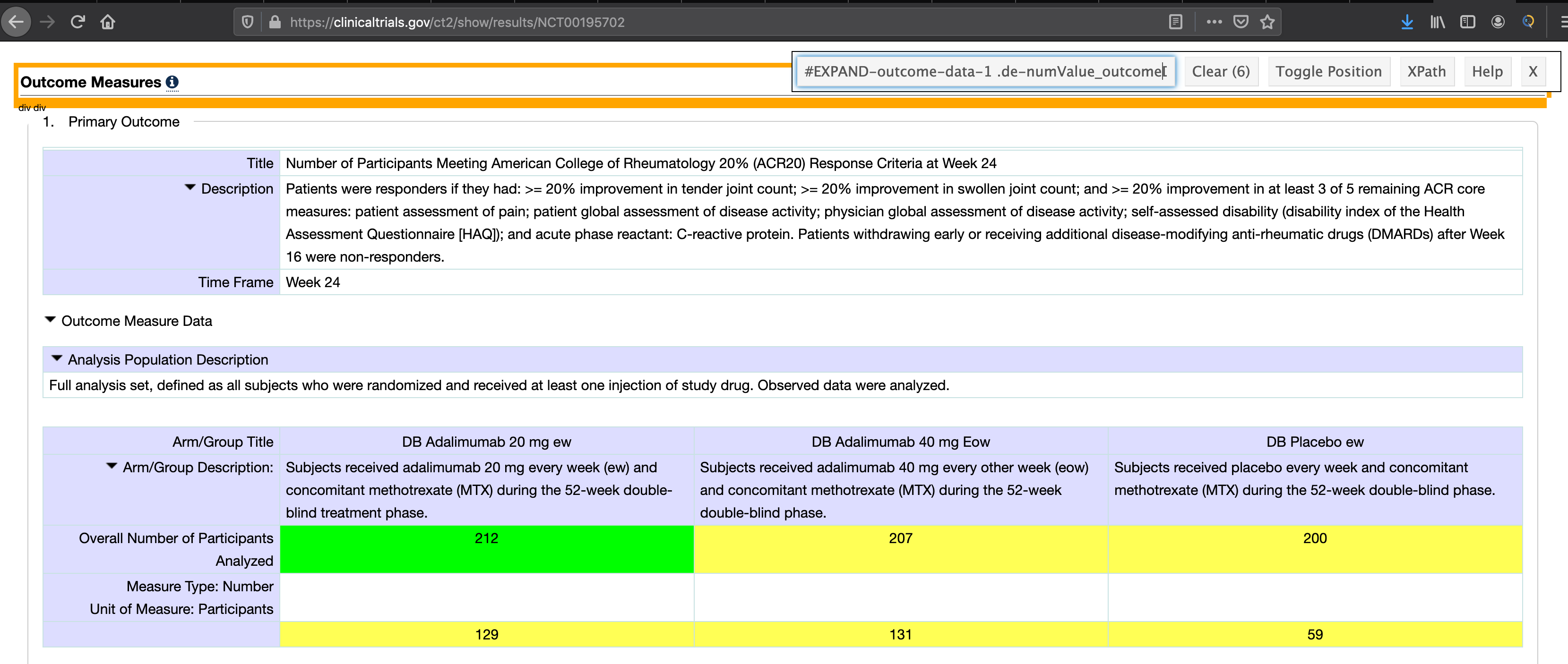
Testing Data Scraping and Transformation to Dataframe
The goal of this portion is to iteratively grab primary outcome data from clinicaltrials.gov, determine if the type of data allows us to calculate a fragility index, then tidy the data into a tibble to allow us to actually calculate it.
We started by testing our code to create a dataframe from a single source. It took quite a few trial and errors to be able to obtain the right form.
Firstly, we attempt to find an identifier relevant to our project that may help us automate the determination of which trial has data eligible for calculating FI.
# test to obtain the particular unit of measure; "participants"
test_url_ctgov <- read_html("https://ClinicalTrials.gov/show/results/NCT00195702") %>%
  html_nodes("#EXPAND-outcome-data-1 .labelSubtle") %>%
  html_text() %>%
  str_replace("Unit of Measure: ", "")
This returns the “unit of measure” of the primary outcome of any given clinical trial. We are particularly looking for outcomes that contain “participants”. We do this because we are looking for trials that have a primary endpoint that involves a standard 2x2 table, which will allow us to calculate a fisher exact test, which is necessary to calculate the fragility index. Through trial and error, we found “unit of measure” to be the best proxy to filter the data.
Having found a way to detect this, we continued to build our function under the assumption that we have “participants” as our unit of measure.
We obtained the relevant column names:
# pulling the relevant column names that corresponds to the eventual numbers we pulled.
# this always has the first term be "\n    Arm/Group Title \n  ", which we will ignore
col_names_test <- read_html("https://ClinicalTrials.gov/show/results/NCT00195702") %>%
  html_nodes("#EXPAND-outcome-data-1 tbody:nth-child(2) tr:nth-child(1) .de-outcomeLabelCell") %>%
  html_text()

col_names_test
## [1] "\n    Arm/Group Title \n  "
## [2] "\n      DB Adalimumab 20 mg ew    "
## [3] "\n      DB Adalimumab 40 mg Eow    "
## [4] "\n      DB Placebo ew    "
The row names, in case we need it as well:
# obtains relevant row names
# ideally this will be participants and the specified units of measure
row_names_test <- read_html("https://ClinicalTrials.gov/show/results/NCT00195702") %>%
  html_nodes("#EXPAND-outcome-data-1 .labelSubtle , #EXPAND-outcome-data-1 tbody:nth-child(2) tr:nth-child(4) .de-outcomeLabelCell") %>%
  html_text()

row_names_test
## [1] "\n    Overall Number of Participants Analyzed   "
## [2] "Unit of Measure: Participants"
And finally, our most important component, which is the number of participants in each group. The code chunks above and below combined detect the number of rows and columns in any clinicaltrials.gov website, grab available data in a vector, then recreate the table in a tidy fashion within R!
# scrape the actual data, with variable table length
content_test <- read_html("https://ClinicalTrials.gov/show/results/NCT00195702") %>%
  html_nodes("#EXPAND-outcome-data-1 .de-numValue_outcomeDataCell") %>%
  html_text() %>%
  as.numeric() %>%                           # cleans our data to contain just the numbers
  matrix(ncol = length(col_names_test[-1]),  # make into a matrix of correct size
         nrow = length(row_names_test),
         byrow = TRUE) %>%
  as_tibble()                                # convert the matrix into a tibble

# add column names to our df
names(content_test) <- col_names_test[-1]

# adds rownames to our tibbles
# a tibble doesnt show rownames when you call it but it is saved into R
rownames(content_test) <- row_names_test

content_test
## # A tibble: 2 x 3
##   `\n      DB Adalimumab 2… `\n      DB Adalimumab 40… `\n      DB Placebo…
## *                     <dbl>                      <dbl>                <dbl>
## 1                       212                        207                  200
## 2                       129                        131                   59
Though it took a while, our code managed to pull the relevant info that we need to manipulate in order to evaluate our fragility indexes. Our next step then, is to be able to map this and make a listcol within our original dataframe.
Building the function with the proper conditions and mapping
Similar to how we approach making the single-url code, we had various trial and error to come up with the function. We start with a simple object that stores our base url and ClinicalTrials.gov Identifier. We iteratively go to each website and extract the “unit of measure” of the primary outcome of the trial and evaluate whether or not it contains “participants” or “patients”; scrape if TRUE, return NA if FALSE.
A slightly different step was to split the content-scraping and data-frame transformation into two separate steps in order to clarify the segmentation.
# function to scrape from url
outcome_extractor <- function(data) {

  # stores our list of urls
  site = read_html(str_c("https://ClinicalTrials.gov/show/results/", data))

  # pulls our "measure" detector
  measure = site %>%
    html_nodes("#EXPAND-outcome-data-1 .labelSubtle") %>%
    html_text() %>%
    str_replace("Unit of Measure: ", "")

  # if/else function that skips to the next url if our measure does not contain "participants" or "patients"
  if (length(measure) == 0) {      # added after bug found; accounts for length = 0
    NA
  } else if (!str_detect(measure, "[pP]articipants|[pP]atients")) {
    NA            # returns NA if it doesn't exist
  } else {

    # pulls relevant column names
    col_names = site %>%
      html_nodes("#EXPAND-outcome-data-1 tbody:nth-child(2) tr:nth-child(1) .de-outcomeLabelCell") %>%
      html_text()

    # pulls row names (might be unnecessary)
    row_names = site %>%
      html_nodes("#EXPAND-outcome-data-1 .labelSubtle , #EXPAND-outcome-data-1 tbody:nth-child(2) tr:nth-child(4) .de-outcomeLabelCell") %>%
      html_text()

    # pulls the actual numbers (content)
    content = site %>%
      html_nodes(".de-numValue_outcomeDataCell") %>%
      html_text() %>%
      as.numeric()

    # makes a dataframe using matrix
    df = matrix(content,
                ncol = length(col_names[-1]),
                nrow = length(row_names),
                byrow = TRUE) %>%
      as_tibble()

    # adds column names
    names(df) <- col_names[-1]
    rownames(df) <- row_names

    # returns the df output
    df
  }
}
We then test this by scraping our .csv file, ctgov_test_API.csv located inside our data folder (loaded earlier) and map our newly-made function. A critical step after we tested this was that we need to filter our NA for our listcol to appear properly.
# testing our function using purrr::map function.
mapped_ctgov_scrape_test <- ctgov_scrape_test %>%
  mutate(
    scrape_data = map(nct_id, outcome_extractor)
  ) %>%
  filter(!is.na(scrape_data))               # necessary step to clear out the NA rows.
We then checked those trials that contain 2x2 table from our original file with stricter search criteria but we only found 6 (uh-oh). After realizing the situation we were in (yikes) and the amount of data we were likely able to get using the initial hypothesis (not enough), we expanded our initial search options to any completed phase 3 clinical trials.
Mapping our 10,000 dataset
Now that we expanded our scope, we use our working function on our new data source, ctgov_10k_API. This however, takes about 30-40 minutes to compile.
Note: During one of our tries, we realize that there’s an extra element in the “outcome measures” that we failed to take into account; character(0). This is different from NA. We had to debug this for a while to make our function work by adding another condition: if(length(input) == 0), which returns NA if TRUE.
ctgov_10k_df <- read_csv("./data/ctgov_10k_API.csv") %>%              # read csv
  janitor::clean_names() %>%
  mutate(
    url = str_replace(url, "https://ClinicalTrials.gov/show/", "")    # keep trial ID only
  ) %>%
  rename("nct_id" = url) %>%
  select(rank, nct_id, title, conditions, interventions) %>%
  filter(str_detect(interventions, "Placebo"))

# testing our function using purrr::map function.
ctgov_10k_scraped <- ctgov_10k_df %>%
  mutate(
    scrape_data = map(nct_id, outcome_extractor)
  ) %>%
  filter(!is.na(scrape_data))               # necessary step to clear out the NA rows.
After all this, our resulting viable dataset is 620 datasets that each contains the primary outcomes of interest. There are roughly 394 unique conditions found using distinct() function.
Cleaning the Scraped Dataset
After scraping the hard numbers in the scrape_data column, we found that according to clinicaltrials.gov output issue, the html node doesn’t necessarily extract the information we want. Therefore, we have no choice but to filter out trials that did not capture this info (contains NA) from our dataset.
# left as _test for now, change it back to ctgov_10k_scraped later
ctgov_10k_scraped <- ctgov_10k_scraped %>%
  mutate(
    nainside = map_chr(scrape_data, anyNA))

# show the count of those with NA vs without
ctgov_10k_scraped %>%
  count(nainside)
## # A tibble: 2 x 2
##   nainside     n
##   <chr>    <int>
## 1 FALSE      274
## 2 TRUE       346
As shown above, we have 274 intact datasets for FI analysis. We further filter this by selecting only the datasets that has number of participants as unit of measure.
# select those doesn't contain NAs
clean_ctgov_df <- ctgov_10k_scraped %>%
  filter(nainside == FALSE)

# function to obtain unit of measure
unit_detector = function(data) {

  site = read_html(str_c("https://ClinicalTrials.gov/show/results/", data))  # stores url

  measure = site %>%                                                         # grabs unit of measure
    html_nodes("#EXPAND-outcome-data-1 .labelSubtle") %>%
    html_text() %>%
    str_replace("Unit of Measure:", "")

  return(measure)                                                            # returns as character
}

# adding unit of measure to the dataset
clean_ctgov_df <- clean_ctgov_df %>%
  mutate(
    units = map_chr(nct_id, unit_detector)
  )

# remove those containing percent/proportions in their unit of measure
# as well as those that are not 2x2 tables
new_df <- clean_ctgov_df %>%
  filter(!str_detect(units, "[pP]ercent|[pP]ercentage|[pP]roportion")) %>%
  mutate(
    nrow = map_dbl(scrape_data, nrow),                  # counts rows in each of our scraped data
    ncol = map_dbl(scrape_data, ncol)                   # counts columns in each of our scraped data
  ) %>%
  filter(ncol == 2 & nrow == 2)
After all these, we now have trials with number of patients as unit of measures and we further filtered out those that have complicated results more than 2 arms. The resulting dataset has 39 trials in it. A quick distinct() suggests each trials are for unique conditions/disease.
We further tried to extract, modify, access the dataframe we made for each trials but despite numerous attempts, none worked. This is likely due to how purrr::map functions with list versus tibbles. Therefore, we have no choice but to manually type out the 39 studies and save it as a new csv file. Since we made it manually, we made sure to split the trial arms into separate columns.
# some miracle happened!!!
manual <- read_csv("./data/FI2by2_manual.csv")

# rejoin the results back to the orignial data
final_df <- left_join(new_df, manual, by = "nct_id") %>%
  select(everything(), -nrow, -ncol, -nainside, -scrape_data)
We thought we were safe but more issues await. Mapping the function fragilityindex::fragility.index, (R documentation here) appears to use a lot of “workspace” in RStudio, thereby preventing us from mapping fragility.index to each row. As a result, we had to make a for loop.
# stores nct_id
nct = c()

# stores result of fragility.index function
FI = c()

# the loop function
for (i in 1:nrow(final_df)) {
  # stores nct_id of each
  nct[i] = final_df$nct_id[i]

  # stores the FI result
  FI[i] = fragility.index(intervention_event = final_df$effective_trt[i],
                          control_event = final_df$effective_placebo[i],
                          intervention_n = final_df$total_number_trt[i],
                          control_n = final_df$total_number_placebo[i])
}

# temporary dataframe to turn our loop result into a df
temp_df <- tibble(
  nct_id = nct,
  FI = as.numeric(FI)
)

# left join the final results
clean_final_df <- left_join(final_df, temp_df, by = "nct_id")
After all of the above, we finally have a dataframe that has just enough data to get a preliminary look at the fragility index. Our final dataset contains 39 trials with 10 relevant variables:
nct_id: trial ID from clinicaltrials.govtitle: title for the trial submitted to clinicaltrials.govconditions: trial’s condition/disease of interestinterventions: interventions done in the trialunits: units of measure (filtered for number of participants)total_number_trt: sample size in the treatment grouptotal_number_placebo: sample size in the control groupeffective_trt: those that developed a response in treatment groupeffective_placebo: those that developed a response in control groupFI: fragility index calculated using fragilityindex::fragility.index
EDA for Fragility Index
summary(clean_final_df$FI)
##    Min. 1st Qu.  Median    Mean 3rd Qu.    Max.
##   0.000   0.000   0.000   6.949   1.000  67.000
A quick summary() reveals another, unexpected issue: 28 of our data appears to be 0, which is about 71.79% of our data. This is likely because these trials already has statistically non-significant results in the first place.
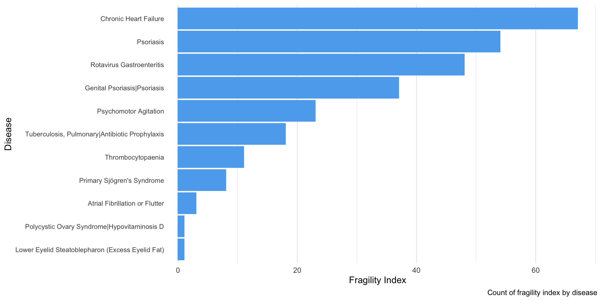
Given our limited data we obtained, we could only create general descriptive table of FI corresponding to the disease conditions.
# quick review of available FI data > 0
clean_final_df %>%
  select(title, conditions, interventions, FI) %>%
  filter(FI != 0) %>%
  arrange(desc(FI)) %>%
  knitr::kable("html",
         caption = "Clinical Trials and their Fragility Index")
Clinical Trials and their Fragility Index
|
title
|
conditions
|
interventions
|
FI
|
|
Effects of Ivabradine on Cardiovascular Events in Patients With Moderate to Severe Chronic Heart Failure and Left Ventricular Systolic Dysfunction. A Three-year International Multicentre Study
|
Chronic Heart Failure
|
Drug: Ivabradine|Drug: Placebo
|
67
|
|
Study of Secukinumab With 2 mL Pre-filled Syringes
|
Psoriasis
|
Drug: Placebo|Drug: Secukinumab 2 mL form|Drug: Secukinumab 1 mL form
|
54
|
|
Efficacy, Safety, and Immunogenicity of V260 in Healthy Chinese Infants (V260-024)
|
Rotavirus Gastroenteritis
|
Biological: V260|Biological: Placebo to V260|Biological: OPV|Biological: DTaP
|
48
|
|
A Study of Ixekizumab (LY2439821) in Participants With Moderate-to-Severe Genital Psoriasis
|
Genital Psoriasis|Psoriasis
|
Drug: Ixekizumab|Drug: Placebo
|
37
|
|
Does Intraoperative Clonidine Reduce Post Operative Agitation in Children?
|
Psychomotor Agitation
|
Drug: Clonidine|Drug: Placebo
|
23
|
|
Prevention of Tuberculosis in Prisons
|
Tuberculosis, Pulmonary|Antibiotic Prophylaxis
|
Drug: Isoniazid 900 milligrams|Drug: Placebo
|
18
|
|
A Study of Eltrombopag or Placebo in Combination With Azacitidine in Subjects With International Prognostic Scoring System (IPSS) Intermediate-1, Intermediate-2 or High-risk Myelodysplastic Syndromes (MDS)
|
Thrombocytopaenia
|
Drug: Eltrombopag|Drug: Azacitidine|Drug: Placebo
|
11
|
|
Safety, Pharmacokinetics, and Preliminary Efficacy Study of CDZ173 in Patients With Primary Sjögren’s Syndrome
|
Primary Sjögren’s Syndrome
|
Drug: CDZ173|Drug: Placebo
|
8
|
|
Safety and Efficacy of Vanoxerine for the Conversion of Subjects With Recent Onset Atrial Fibrillation or Flutter to Normal Sinus Rhythm
|
Atrial Fibrillation or Flutter
|
Drug: Vanoxerine HCl|Drug: Placebo
|
3
|
|
The Effect of Vitamin D Supplementation Among Overweight Jordanian Women With Polycystic Ovary Syndrome (PCOS)
|
Polycystic Ovary Syndrome|Hypovitaminosis D
|
Drug: 50,000 IU vitamin D3|Drug: Placebo
|
1
|
|
Phase 2 Study of XAF5 (XOPH5) Ointment for Reduction of Excess Eyelid Fat (Steatoblepharon)
|
Lower Eyelid Steatoblepharon (Excess Eyelid Fat)
|
Drug: XOPH5 Ointment|Drug: Placebo
|
1
|
A visualization of this “trend” in FI is shown below:
# barplot according to corresponding disease/ treatment
clean_final_df %>%
  filter(FI != 0) %>%
  arrange(desc(FI)) %>%
  ggplot(aes(x = reorder(conditions, FI), y = FI)) +
  geom_bar(stat = "identity", color = "steelblue2", fill = "steelblue2") +
  coord_flip() +                                              # flip x-y to better "stratify" categories
  theme(legend.position = "none",                             # remove legends
        axis.text.y =
          element_text(hjust = 1, vjust = 0.5,                # adjusts the hor/ver alignment of y-variables
                       size = 8,                              # resize text size and rotate at an angle
                       margin = margin(0, -10, 0, 0)),        # reduce margin to close gap between label/graph
        panel.grid.major.y = element_blank()                  # remove horizontal lines to improve readability
        ) +
  labs(x = "Disease", y = "Fragility Index",
       caption = "Count of fragility index by disease")